

 Es
Es  Fr
Fr  Pt
Pt  En
En 

Creating Orthophotoplans
 Ribbon: Point Clouds > Aerial Laser Scanning >
  Creating Orthophotoplans
Menu: Point Clouds >  Creating Orthophotoplans
Toolbar: Aerial Laser Scanning >
 Command line: PC_MOSAIC
 This is a trial version. The command is currently in a testing mode and may be changed or removed in future releases.
The command is designed to create orthophotoplans from a set of overlapping images.
An orthophotoplan is a raster image of an area in a given cartographic coordinate system.
The source data are the images themselves, camera parameters, and the camera’s trajectory with the moments of photography. Processing results in one or more orthophotoplans in GeoTIFF format.
To create orthophotoplans, the following processing steps should be completed:
1. Creating a project.
2. Editing manually the photo cut lines created automatically during project creation.
3. Creating orthophotomap sheet borders.
4. Creating orthophotomaps from sheet borders.
Creating a project
To create a project, click on  in the dialog box that opens.

Here, enter the data required for orthotransformation of images:
· project file name;
· folder with photo files in TIFF format;
· camera file created in the Edit camera properties dialog (PC_EDIT_CAMERA command);
· elevation matrix created in the Create a DEM based on point clouds dialog (PC_CLOUDS_TO_DEM command);
· time-photo file. It is used to search for image exterior orientation elements in trajectory files. It is a text file containing the image file name and time, line by line, without the path or extension;
· folder containing trajectory files in text or TRJ format;
· enter the pixel size of the generated orthophotos, which will be visible in the main program window after the project is created. They are needed as a base for digitizing the cuts.
|
|
Note |
|
When working with a project, images are loaded into RAM, so it is not recommended to set a small pixel size. However, the pixel size should be sufficient to reliably recognize objects in the images. In most cases, a pixel size of 0.5 – 1 meter will be sufficient. |

Once processing is complete, the transformed images with cuts and a sheet border created based on the overall dimensions of the images will be loaded into the main window.
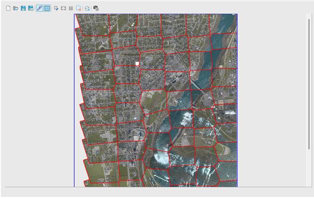
To navigate the image, drag the mouse while holding down the mouse wheel, and to zoom, rotate the mouse wheel.
Editing cuts
In aerial photography, a single point appears in multiple images. Therefore, when creating an ortho], the problem arises of determining which image to use for the pixel color.
Since terrain distortion in an image increases with distance from the image center, the best choice is an image in which the point is located at a minimum distance from the center. Based on this requirement, Voronoi polygons are a good approximation for creating initial cutlines. They need to be edited for two reasons:
· when creating a DEM, the DEM is based on the ground surface, ignoring objects on the surface. Therefore, when a cutline intersects high-altitude objects in the orthomosaic, discrepancies will be visible due to the different directions of object displacement in different images. Therefore, the cutline should run along the ground surface.
· due to errors in the orientation elements, there will inevitably be slight shifts in the cuts, so the cut should ideally pass through inconspicuous and uninformative areas – forests, fields, etc.
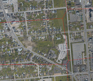
Cut editing mode is activated by pressing the  button on the toolbar.

|
|
Note |
|
|
To expand the outline of a photo cut, start and finish digitizing a polygon within the cut. Points are added by clicking the left mouse button. |
|
|
Finish digitizing by double-clicking the mouse. Once digitizing is complete, the polygon will be added to the cut from which digitizing began, and the polygon will be removed from adjacent cuts.
|
|
Note |
|
|
The cut should be made within the boundaries of its image, not in areas that do not overlap with adjacent images. Failure to comply with this requirement will result in unfilled areas in the resulting photomosaic. |
|
|
To help navigate the image boundaries, they are displayed when hovering over the image while holding down the Shift key.
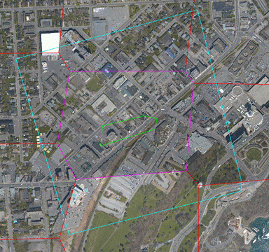
When digitizing an expanding polygon, you can use hotkeys:
· Backspace deletes the last point;
· Esc deletes all points;
· Ctrl+Z deletes the last cut update;
· Spacebar erases the outer and inner boundaries of the image.
The same commands can be accessed through the context menu by right-clicking.
Creating sheet frames
The program offers three frame creation modes:
 Creates a single sheet for all photos based on the overall dimensions of the photos. When creating a project, the sheet is created in this mode.
 The user specifies the dimensions of a single sheet by the selected frame using a rubber rectangle.
 Opens the Cut into sheets dialog.
The dialog specifies the sheet size, the prefix for the name of the orthomosaic being created, and the sheet numbering order. After clicking the Apply button, sheets are created for the entire image coverage area.
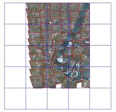
After creation, extra sheets can be deleted by enabling the delete sheet mode using the  button. When deleting sheets, the last sheet cannot be deleted to ensure that the transformation boundaries are always defined.
Creating orthophotoplans from sheet frames
The orthotransformation dialog is opened by clicking the  button in the toolbar.
In the orthorectification dialog, enter data that supplement the parameters entered when creating the project.
The folder for the generated orthomosaics or the name of the orthomosaic being created, depending on whether multiple sheets or a single sheet are being created. All files in the selected folder are deleted before processing.
Raster DEM
When the dialog is first opened, the DEM selected when creating the project is used. You can change it if you selected a DEM with a larger element size when creating the project to speed up project creation.
Pixel Size
Enter the desired pixel size for the generated orthophotoplans.
Blur Radius
Specify the blur radius for image cuts to reduce their visibility. Entering 0 means no blurring.
Image and DEM Interpolation (Nearest Neighbor or Bilinear)
Determines the method for interpolating pixel color and elevation from the DEM. Bilinear interpolation provides better visual quality but slightly slower processing.
Color Balancing
Images covering the survey area have slight color differences. To eliminate these, two color balancing strategies are used.
Global balancing calculates a single color transformation for all pixels in a single image. Local balancing determines pixel color changes based on an analysis of the colors of neighboring pixels from all overlapping images.
Global balancing equalizes the average background of images, while local balancing eliminates local discrepancies at cutlines.
The best results are achieved by using both balancing methods. If both modes are disabled, the pixel colors of the orthomosaic are copied from the corresponding image without modification.
If the image contains large areas of shadow or highlight, they will affect the color transformation parameters of both global and local balancing. To eliminate their influence, specify the shadow and highlight colors in the Shadow if the color is smaller and Highlight if the color is larger fields. The condition is considered met if all three color components match the specified value. If there are no large areas of shadow and highlight, then specify values of 0 and 255.
After color balancing, the total color range no longer corresponds to the natural encoding from 0 to 255.
The classic color normalization method is a linear color transformation based on the index of the first and last non-zero histogram values. This typically results in a low-contrast image.
To improve contrast, it’s better to use the values obtained by the first and last intersection of the horizontal line with the histogram.
The height of the line above the horizontal axis of the graph is specified as a percentage of the maximum histogram value in the Histogram Clipping (%) field.
|
|
Note |
|
|
In most cases, 1-2% is sufficient. If you specify 0, the color is converted based on the index of the first and last non-zero histogram values. |
|
|
By default, the two options are included:  Show photo cuts and
  Show sheet borders.